Example - Zonal Statistics
This is useful in the case where you want to get regional statistics for a raster.
[1]:
import geopandas
import numpy
import rioxarray
import xarray

from geocube.api.core import make_geocube

%matplotlib inline
Create the data mask by rasterizing the unique ID of the vector data
See docs for make_geocube
[2]:
# This assumes you are running this example from a clone of
# https://github.com/corteva/geocube/
# You could also use the full path:
# https://raw.githubusercontent.com/corteva/geocube/master/test/test_data/input/soil_data_group.geojson
ssurgo_data = geopandas.read_file("../../test/test_data/input/soil_data_group.geojson")
ssurgo_data = ssurgo_data.loc[ssurgo_data.hzdept_r==0]
# convert the key to group to the vector data to an integer as that is one of the
# best data types for this type of mapping. If your data is not integer,
# then consider using a mapping of your data to an integer with something
# like a categorical dtype.
ssurgo_data["mukey"] = ssurgo_data.mukey.astype(int)
[3]:
# load in source elevation data subset relevant for the vector data
elevation = rioxarray.open_rasterio(
    "https://prd-tnm.s3.amazonaws.com/StagedProducts/Elevation/13/TIFF/current/n42w091/USGS_13_n42w091.tif", masked=True
).rio.clip(
    ssurgo_data.geometry.values, ssurgo_data.crs, from_disk=True
).sel(band=1).drop("band")
elevation.name = "elevation"
[4]:
out_grid = make_geocube(
    vector_data=ssurgo_data,
    measurements=["mukey"],
    like=elevation, # ensure the data are on the same grid
)
[5]:
# merge the two together
out_grid["elevation"] = (elevation.dims, elevation.values, elevation.attrs, elevation.encoding)
out_grid
[5]:
<xarray.Dataset>
Dimensions:      (y: 178, x: 178)
Coordinates:
  * y            (y) float64 41.5 41.5 41.5 41.5 ... 41.48 41.48 41.48 41.48
  * x            (x) float64 -90.6 -90.6 -90.6 -90.6 ... -90.58 -90.58 -90.58
    spatial_ref  int64 0
Data variables:
    mukey        (y, x) float64 1.988e+05 1.988e+05 ... 1.987e+05 1.987e+05
    elevation    (y, x) float64 173.7 172.0 171.1 170.6 ... 181.0 181.2 181.4
xarray.Dataset
- y: 178
- x: 178
- y(y)float6441.5 41.5 41.5 ... 41.48 41.48
- axis :
- Y
- long_name :
- latitude
- standard_name :
- latitude
- units :
- degrees_north
array([41.499861, 41.499769, 41.499676, 41.499583, 41.499491, 41.499398, 41.499306, 41.499213, 41.49912 , 41.499028, 41.498935, 41.498843, 41.49875 , 41.498657, 41.498565, 41.498472, 41.49838 , 41.498287, 41.498194, 41.498102, 41.498009, 41.497917, 41.497824, 41.497731, 41.497639, 41.497546, 41.497454, 41.497361, 41.497269, 41.497176, 41.497083, 41.496991, 41.496898, 41.496806, 41.496713, 41.49662 , 41.496528, 41.496435, 41.496343, 41.49625 , 41.496157, 41.496065, 41.495972, 41.49588 , 41.495787, 41.495694, 41.495602, 41.495509, 41.495417, 41.495324, 41.495231, 41.495139, 41.495046, 41.494954, 41.494861, 41.494769, 41.494676, 41.494583, 41.494491, 41.494398, 41.494306, 41.494213, 41.49412 , 41.494028, 41.493935, 41.493843, 41.49375 , 41.493657, 41.493565, 41.493472, 41.49338 , 41.493287, 41.493194, 41.493102, 41.493009, 41.492917, 41.492824, 41.492731, 41.492639, 41.492546, 41.492454, 41.492361, 41.492269, 41.492176, 41.492083, 41.491991, 41.491898, 41.491806, 41.491713, 41.49162 , 41.491528, 41.491435, 41.491343, 41.49125 , 41.491157, 41.491065, 41.490972, 41.49088 , 41.490787, 41.490694, 41.490602, 41.490509, 41.490417, 41.490324, 41.490231, 41.490139, 41.490046, 41.489954, 41.489861, 41.489769, 41.489676, 41.489583, 41.489491, 41.489398, 41.489306, 41.489213, 41.48912 , 41.489028, 41.488935, 41.488843, 41.48875 , 41.488657, 41.488565, 41.488472, 41.48838 , 41.488287, 41.488194, 41.488102, 41.488009, 41.487917, 41.487824, 41.487731, 41.487639, 41.487546, 41.487454, 41.487361, 41.487269, 41.487176, 41.487083, 41.486991, 41.486898, 41.486806, 41.486713, 41.48662 , 41.486528, 41.486435, 41.486343, 41.48625 , 41.486157, 41.486065, 41.485972, 41.48588 , 41.485787, 41.485694, 41.485602, 41.485509, 41.485417, 41.485324, 41.485231, 41.485139, 41.485046, 41.484954, 41.484861, 41.484769, 41.484676, 41.484583, 41.484491, 41.484398, 41.484306, 41.484213, 41.48412 , 41.484028, 41.483935, 41.483843, 41.48375 , 41.483657, 41.483565, 41.483472]) - x(x)float64-90.6 -90.6 -90.6 ... -90.58 -90.58
- axis :
- X
- long_name :
- longitude
- standard_name :
- longitude
- units :
- degrees_east
array([-90.599861, -90.599769, -90.599676, -90.599583, -90.599491, -90.599398, -90.599306, -90.599213, -90.59912 , -90.599028, -90.598935, -90.598843, -90.59875 , -90.598657, -90.598565, -90.598472, -90.59838 , -90.598287, -90.598194, -90.598102, -90.598009, -90.597917, -90.597824, -90.597731, -90.597639, -90.597546, -90.597454, -90.597361, -90.597269, -90.597176, -90.597083, -90.596991, -90.596898, -90.596806, -90.596713, -90.59662 , -90.596528, -90.596435, -90.596343, -90.59625 , -90.596157, -90.596065, -90.595972, -90.59588 , -90.595787, -90.595694, -90.595602, -90.595509, -90.595417, -90.595324, -90.595231, -90.595139, -90.595046, -90.594954, -90.594861, -90.594769, -90.594676, -90.594583, -90.594491, -90.594398, -90.594306, -90.594213, -90.59412 , -90.594028, -90.593935, -90.593843, -90.59375 , -90.593657, -90.593565, -90.593472, -90.59338 , -90.593287, -90.593194, -90.593102, -90.593009, -90.592917, -90.592824, -90.592731, -90.592639, -90.592546, -90.592454, -90.592361, -90.592269, -90.592176, -90.592083, -90.591991, -90.591898, -90.591806, -90.591713, -90.59162 , -90.591528, -90.591435, -90.591343, -90.59125 , -90.591157, -90.591065, -90.590972, -90.59088 , -90.590787, -90.590694, -90.590602, -90.590509, -90.590417, -90.590324, -90.590231, -90.590139, -90.590046, -90.589954, -90.589861, -90.589769, -90.589676, -90.589583, -90.589491, -90.589398, -90.589306, -90.589213, -90.58912 , -90.589028, -90.588935, -90.588843, -90.58875 , -90.588657, -90.588565, -90.588472, -90.58838 , -90.588287, -90.588194, -90.588102, -90.588009, -90.587917, -90.587824, -90.587731, -90.587639, -90.587546, -90.587454, -90.587361, -90.587269, -90.587176, -90.587083, -90.586991, -90.586898, -90.586806, -90.586713, -90.58662 , -90.586528, -90.586435, -90.586343, -90.58625 , -90.586157, -90.586065, -90.585972, -90.58588 , -90.585787, -90.585694, -90.585602, -90.585509, -90.585417, -90.585324, -90.585231, -90.585139, -90.585046, -90.584954, -90.584861, -90.584769, -90.584676, -90.584583, -90.584491, -90.584398, -90.584306, -90.584213, -90.58412 , -90.584028, -90.583935, -90.583843, -90.58375 , -90.583657, -90.583565, -90.583472]) - spatial_ref()int640
- crs_wkt :
- GEOGCS["NAD83",DATUM["North_American_Datum_1983",SPHEROID["GRS 1980",6378137,298.257222101004,AUTHORITY["EPSG","7019"]],AUTHORITY["EPSG","6269"]],PRIMEM["Greenwich",0],UNIT["degree",0.0174532925199433,AUTHORITY["EPSG","9122"]],AXIS["Latitude",NORTH],AXIS["Longitude",EAST],AUTHORITY["EPSG","4269"]]
- semi_major_axis :
- 6378137.0
- semi_minor_axis :
- 6356752.314140356
- inverse_flattening :
- 298.257222101004
- reference_ellipsoid_name :
- GRS 1980
- longitude_of_prime_meridian :
- 0.0
- prime_meridian_name :
- Greenwich
- geographic_crs_name :
- NAD83
- grid_mapping_name :
- latitude_longitude
- spatial_ref :
- GEOGCS["NAD83",DATUM["North_American_Datum_1983",SPHEROID["GRS 1980",6378137,298.257222101004,AUTHORITY["EPSG","7019"]],AUTHORITY["EPSG","6269"]],PRIMEM["Greenwich",0],UNIT["degree",0.0174532925199433,AUTHORITY["EPSG","9122"]],AXIS["Latitude",NORTH],AXIS["Longitude",EAST],AUTHORITY["EPSG","4269"]]
array(0)
- mukey(y, x)float641.988e+05 1.988e+05 ... 1.987e+05
- name :
- mukey
- long_name :
- mukey
- _FillValue :
- nan
array([[198754., 198754., 198754., ..., 198750., 198750., 198750.], [198754., 198754., 198754., ..., 198750., 198750., 198750.], [198754., 198754., 198754., ..., 198750., 198750., 198750.], ..., [198754., 198754., 198754., ..., 198724., 198724., 198724.], [198754., 198754., 198754., ..., 198724., 198724., 198724.], [198754., 198754., 198754., ..., 198724., 198724., 198724.]]) - elevation(y, x)float64173.7 172.0 171.1 ... 181.2 181.4
- LAYER_TYPE :
- athematic
- RepresentationType :
- ATHEMATIC
- STATISTICS_MAXIMUM :
- 284.1125793457
- STATISTICS_MEAN :
- 213.62414075786
- STATISTICS_MINIMUM :
- 83.762252807617
- STATISTICS_STDDEV :
- 22.778435029777
- STATISTICS_VALID_PERCENT :
- 100
- scale_factor :
- 1.0
- add_offset :
- 0.0
- long_name :
- Layer_1
array([[173.67080688, 171.96047974, 171.08390808, ..., 172.10124207,
        172.2388916 , 171.97241211],
       [172.68327332, 171.44102478, 170.65075684, ..., 172.20561218,
        172.33590698, 172.00927734],
       [171.81083679, 170.66856384, 170.29721069, ..., 171.5133667 ,
        171.62541199, 171.84867859],
       ...,
       [175.94241333, 176.07365417, 176.73553467, ..., 181.040802  ,
        181.30989075, 181.42185974],
       [176.61058044, 176.91845703, 177.03279114, ..., 181.06401062,
        181.11106873, 181.30020142],
       [176.23300171, 176.77012634, 177.17182922, ..., 180.96748352,
        181.20977783, 181.39945984]])
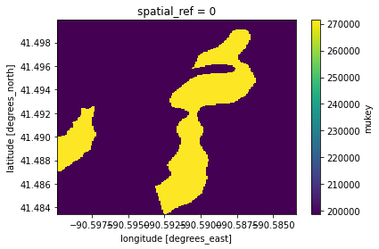
[6]:
out_grid.mukey.plot.imshow()
[6]:
<matplotlib.image.AxesImage at 0x7f2dd5398550>
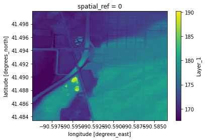
[7]:
out_grid.elevation.plot()
[7]:
<matplotlib.collections.QuadMesh at 0x7f2dd5282ed0>
Get the elevation statistics of each region using the mask
[8]:
grouped_elevation = out_grid.drop("spatial_ref").groupby(out_grid.mukey)
grid_mean = grouped_elevation.mean().rename({"elevation": "elevation_mean"})
grid_min = grouped_elevation.min().rename({"elevation": "elevation_min"})
grid_max = grouped_elevation.max().rename({"elevation": "elevation_max"})
grid_std = grouped_elevation.std().rename({"elevation": "elevation_std"})
[9]:
zonal_stats = xarray.merge([grid_mean, grid_min, grid_max, grid_std]).to_dataframe()
zonal_stats
[9]:
| elevation_mean | elevation_min | elevation_max | elevation_std | |
|---|---|---|---|---|
| mukey | ||||
| 198692.0 | 173.130925 | 169.394562 | 188.442505 | 3.307044 |
| 198714.0 | 175.045866 | 170.214157 | 179.716675 | 2.150987 |
| 198724.0 | 179.931131 | 178.237244 | 181.490387 | 0.630699 |
| 198750.0 | 176.187118 | 167.951233 | 190.138763 | 3.815206 |
| 198754.0 | 171.633084 | 167.610321 | 181.611298 | 2.997591 |
| 271425.0 | 167.974433 | 167.951233 | 168.653015 | 0.079769 |
| 271431.0 | 176.718101 | 170.258133 | 180.460220 | 2.731732 |
[10]:
ssurgo_data = ssurgo_data.merge(zonal_stats, on="mukey")
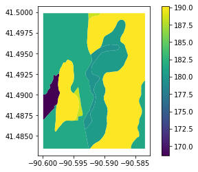
[11]:
ssurgo_data.plot(column="elevation_mean", legend=True)
[11]:
<AxesSubplot:>
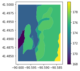
[12]:
ssurgo_data.plot(column="elevation_max", legend=True)
[12]:
<AxesSubplot:>